Application to Transmission Problems with Multiple Junctions

It is easy to define time-harmonic acoustic and electromagnetic scattering problems in piece-wise constant homogeneous media using a chunkgraph object and a helper routine available in chunkie. This includes domains with multiple junctions and an arbitrary nesting of regions defining the dielectric media. Suppose that the dielectric region consists of regions \(\Omega_{j}\), \(j=2,\ldots n_{r}\), and let \(\Omega_{1} = \mathbb{R}^{2} \setminus \cup_{j=2}^{n_{r}} \overline{\Omega_{j}}\) denote the exterior region. Let \(\varepsilon_{j}\) denote the permittivity and let \(k_{j}\) denote the wavenumber in \(\Omega_{j}\). Let \(\Gamma_{\ell}\), \(\ell=1,2,\ldots n_{e}\) denote the edges (possibly curved) in the chunkgraph, and let \(r_{\ell,\pm}\) denote the index of the region numbers pointing in the positive and negative normal direction to the edge respectively.

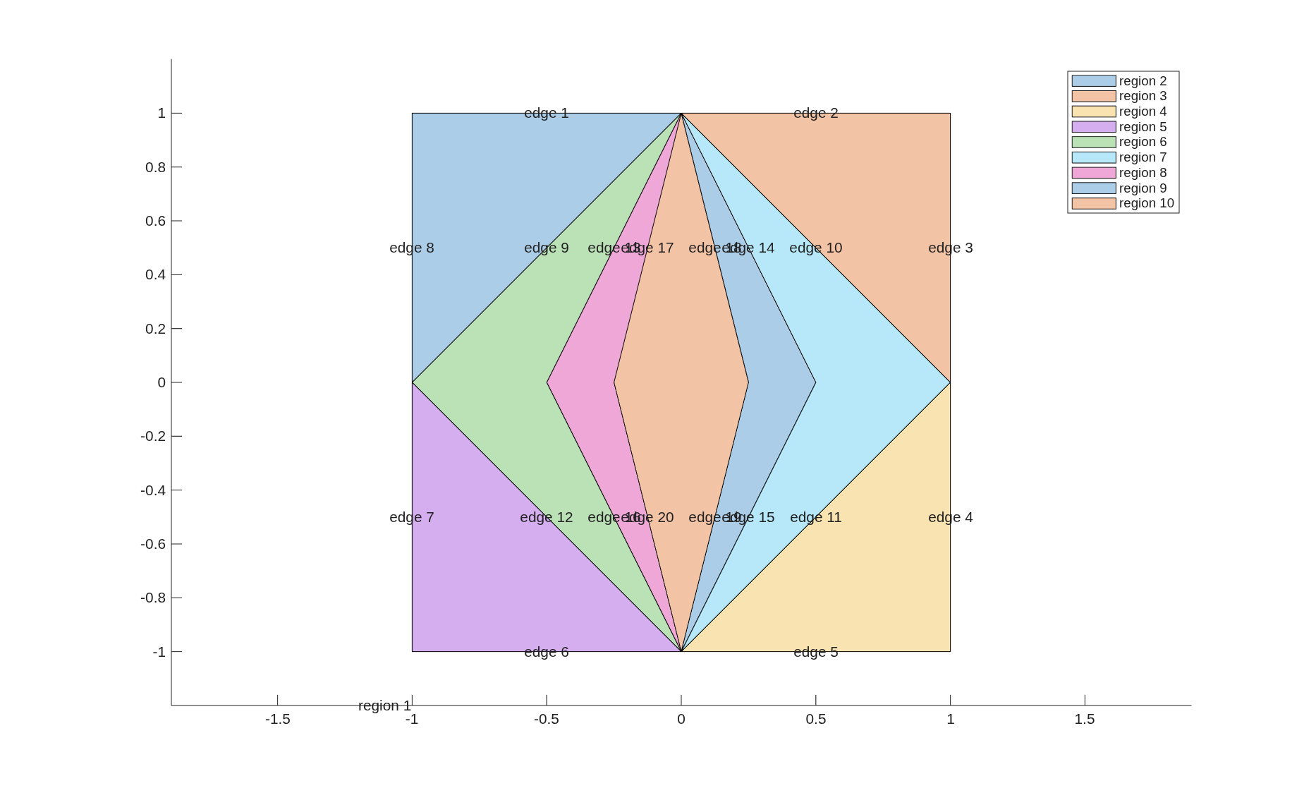
Consider the following domain consisting of \(9\) dielectrics. We use the plot_regions functionality of the chunkgraph to identify its regions and edges.

% define verts
verts_out = [[1;1],[1;-1],[-1;-1],[-1;1]];
verts_in = [[0;1],[1;0],[0;-1],[-1;0]];
verts_in2 = [[1/2;0],[-1/2;0]];
verts_in3 = verts_in2/2;

verts = [verts_out, verts_in, verts_in2, verts_in3];

% geometry will be a series of loops through subsets of vertices
id_vert_out = [5,1,6,2,7,3,8,4];
% call helper function
e2v_out = [id_vert_out;circshift(id_vert_out,1)];

id_vert_in = 5:8;
e2v_in = [id_vert_in;circshift(id_vert_in,1)];

id_vert_in2 = [5,9,7,10];
e2v_in2 =  [id_vert_in2;circshift(id_vert_in2,1)];

id_vert_in3 = [5,11,7,12];
e2v_in3 =  [id_vert_in3;circshift(id_vert_in3,1)];

% combine lists of edges
edge_2_verts = [e2v_out,e2v_in,e2v_in2,e2v_in3];

cparams = [];
cparams.maxchunklen = 4.0/max(zks);
cgrph = chunkgraph(verts,edge_2_verts,[],cparams);
figure(1);
clf
plot_regions(cgrph)
xlim([-2,2])
axis equal 

For electromagnetic scattering, in the transverse electric or transverse magnetic mode, the potentials \(u_{j}\) in \(\Omega_{j}\), \(j=1,\ldots n_{r}\) satisfy the following transmission boundary value problem

\[\begin{split}\begin{aligned} \Delta u_{j} + k_{j}^2 u_{j} &=0 & \textrm{ in } \Omega_{j} \; , j=1,2\ldots n_{r}\\ u_{r_{\ell,+}} - u_{r_{\ell,-}} &= f_{\ell} & \textrm{ on } \Gamma_{\ell} \;, \ell=1,2,\ldots n_{e}\,, \\ \beta_{r_{\ell,+}}\frac{\partial u_{r_{\ell,+}}}{\partial n} - \beta_{r_{\ell,-}}\frac{\partial u_{r_{\ell,-}}}{\partial n} &= g_{\ell} & \textrm{ on } \Gamma_{\ell}\;, \ell=1,2,\ldots n_{e}\,,\\ \sqrt{|x|} \left( \frac{x}{|x|} \cdot \nabla u_{1} - ik_{1} u_{1} \right ) &\to 0 & \textrm{ as } |x|\to \infty \;. \end{aligned}\end{split}\]

Here \(\beta_{j} = 1\) for the transverse magnetic mode and \(\beta_{j} = 1/\varepsilon_{j}\) for the transverse electric mode.

A typical problem of interest is that of computing the scattered field from incident plane waves. In this case, the data \(f_{\ell} = -e^{-ik x\cdot d}\) and \(g_{\ell} = (d\cdot n)e^{-ik x \cdot d}\) are non-zero if and only if they are exposed to the unbounded region, i.e. one of \(r_{\ell,+}\) or \(r_{\ell,-}\) is \(1\), and \(d\) here is the direction of incidence of the plane wave.

Let \(G_{k}\) denote the Green’s function for the Helmholtz equation given by

\[G_{k}(x,y) = \frac{i}{4}H_{0}^{(1)}(k|x-y|)\;.\]

Recall that the single and and double layer potentials are given by

\[\begin{split}\begin{aligned} [S_{k}\sigma](x) &:= \int_\Gamma G_k(x,y) \sigma(y) ds(y)\;, \\ [D_{k}\sigma](x) &:= \int_\Gamma n(y)\cdot \nabla_y G_k(x,y) \sigma(y) ds(y) \;, \end{aligned}\end{split}\]

where \(\Gamma = \cup_{\ell=1}^{n_{e}} \Gamma_{\ell}\).

The potentials \(u_{j}\) can then be defined in terms of the single and double layer potential operators as:

\[\begin{aligned} u_{j}(x) &= \frac{1}{\beta_{j}}[D_{k_{j}}\sigma](x) - [S_{k_{j}}\mu](x) & \textrm{ in } \Omega_{j}\;, \end{aligned}\]

Then, imposing the boundary conditions on this representation results in the following equation for \(\sigma, \mu\):

\[\begin{split}\begin{aligned} \begin{bmatrix} \sigma\\ \mu \end{bmatrix} + \gamma_{\ell}\begin{bmatrix} (\beta_{r_{\ell,-}}D_{k_{r_{\ell,+}}} - \beta_{r_{\ell,+}}D_{k_{r_{\ell,-}}}) & -\beta_{r_{\ell,+}} \beta_{r_{\ell,-}}(S_{k_{r_{\ell,+}}} - S_{k_{r_{\ell,-}}}) \\ (D'_{k_{r_{\ell,+}}} - D'_{k_{r_{\ell,-}}}) & -(\beta_{r_{\ell,+}}S'_{k_{r_{\ell,+}}} - \beta_{r_{\ell,-}}S'_{k_{r_{\ell,-}}}) \end{bmatrix} \begin{bmatrix} \sigma\\ \mu \end{bmatrix} &= \gamma_{\ell}\begin{bmatrix} \beta_{r_{\ell,+}} \beta_{r_{\ell,-}}f_{\ell}\\ g_{\ell} \end{bmatrix} \;\; \textrm{ on } \Gamma_{\ell}\;, \end{aligned}\end{split}\]

for \(\ell=1,2,\ldots n_{e}\) where \(\gamma_{\ell} = \frac{2}{\beta_{r_{\ell,+}} + \beta_{r_{\ell,-}}}\).

Note

Note the single and double layer, and the integral equation are appropriately scaled to ensure that the integral equation is of the form \((I + K)\) as opposed to \(\alpha I + K\) for \(\alpha \neq 1\). The current implementation of the corner compression scheme, RCIP, requires this scaling for solving integral equations on chunkgraphs. This restriction will soon be lifted in an upcoming release of chunkIE, but is required as of the current version.

The chunkermat routine is capable of handling such a problem specification, in which the interaction varies for different pairs of chunkgraph edges. These interactions can be specified as a \(n_{\textrm{edge}}\times n_{\textrm{edge}}\) matrix of kernel objects.

For transmission problems, we also provide a helper routine, chnk.helm2d.transmission_helper, which automates much of the process. This routine only requires the chunkgraph, the wavenumbers \(k_{j}\), the coefficients \(\beta_{j}\) and the regions abutting edges \(r_{\ell,\pm}\) which can be determined using the chunkgraph routine, find_edge_regions. Given this information, the routine returns the kernels for solving the integral equation, the boundary data for scattering from planewaves, and the integral kernels needed to evaluate the solution in any region (for postprocessing/plotting). This simplifies the task of genertaing the system matrix quite a bit, requiring only a few lines of code:

nreg = length(cgrph.regions);

% get region ids of interest programmatically, unbounded is always 1
ids = chunkgraphinregion(cgrph,[0 0.35 -0.35 0.5 -0.5 0.5 0.5 -0.5 -0.5; ...
                                0 0      0    0    0  0.6 -0.6 0.6  -0.6]);

% assign region wavenumbers 
ks = zeros(nreg,1);
ks(1) = zks(1);
ks(ids(1)) = zks(5);
ks(ids(2:3)) = zks(4);
ks(ids(4:5)) = zks(3);
ks(ids(6:end)) = zks(2);

% jump condition coefficients
coefs = ones(1,nreg);


edge_regs = find_edge_regions(cgrph);
% set up parameters for planewave data
opts = [];
opts.bdry_data_type = 'pw';

% build system and get boundary data using the transmission helper
[kerns, bdry_data, kerns_eval] = chnk.helm2d.transmission_helper(cgrph, ...
                                   ks, edge_regs, coefs, opts);
% build system matrix
tic;
[sysmat] = chunkermat(cgrph, kerns);
sysmat = sysmat + eye(size(sysmat,2));
tbuild = toc

The solution can then be plotted in the bulk using chunkerkerneval and the kerns_eval matrix of kernels:

L = 1.5*max(vecnorm(cgrph.r(:,:)));
x1 = linspace(-L,L,300);
[xx,yy] = meshgrid(x1,x1);
targs = [xx(:).'; yy(:).'];
ntargs = size(targs,2);

% evaluate potentials and return region labels
tic;
[uscat, targdomain] = chunkerkerneval(cgrph, kerns_eval, dens, targs);
uscat = reshape(uscat,size(xx));
tplot = toc

% identify points in computational domain
in = chunkerinterior(cgrph,{x1,x1});
out = ~in;

% get incoming solution
uin = zeros(size(xx));
uin(targdomain==1) = planewave([zks(1);0],targs(:,targdomain==1));

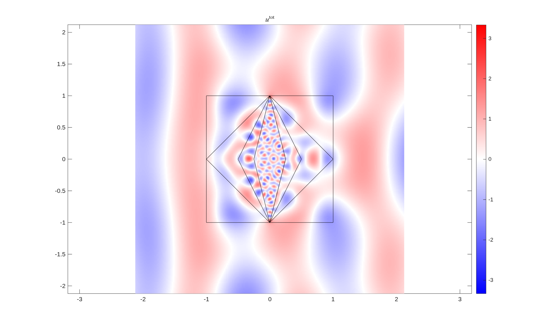
utot = uin + uscat;

umax = max(abs(utot(:))); 
figure(2); clf
h = pcolor(xx,yy,imag(utot)); set(h,'EdgeColor','none'); colorbar
colormap(redblue); clim([-umax,umax]);
hold on 
plot(cgrph,'k')
axis equal
title('$u^{\textrm{tot}}$','Interpreter','latex','FontSize',12)