Solving Standard Boundary Value Problems

ChunkIE uses the integral equation method to solve PDEs. In contrast with finite element methods, where the PDE is typically converted to a weak form, the standard approach for an integral equation method is to select an integral representation of the solution that satisfies the PDE inside the domain a priori. This cannot be done for just any PDE; typically, integral equation methods are limited to constant coefficient, homogeneous PDEs. But when the methods apply, they are efficient and accurate.

The following is a very high level discussion of the main ideas. Some more specific examples are included further below. For more, see, inter alia, [Rok1985], [CK2013], [GL1996], and [Poz1992].

Let \(\Omega\) be a domain with boundary \(\Gamma\). Suppose that we are interested in the solution of the boundary value problem

\[\begin{split}\begin{aligned} \mathcal{L} u &= 0 & \textrm{ in } \Omega \; ,\\ \mathcal{B} u &= f & \textrm{ on } \Gamma \; , \end{aligned}\end{split}\]

where \(\mathcal{L}\) is a linear, constant coefficient PDE operator and \(\mathcal{B}\) is a linear trace operator that restricts \(u\), or some linear operator applied to \(u\), to the boundary.

Suppose that \(G\) is the Green function for \(\mathcal{L}\) and let \(K\) be an integral kernel that is a linear operator applied to \(G\). Then, \(u\) can be represented as a layer potential, i.e. it can be written in the form

\[u(x) = \int_\Gamma K(x,y) \sigma(y) \, ds(y) \; ,\]

which has the property that \(u\) automatically solves the PDE for any choice of density \(\sigma\) (defined on the boundary alone). The idea is to then solve for a specific \(\sigma\) for which the boundary condition holds:

\[\mathcal{B} \left [ \int_\Gamma K(\cdot,y)\sigma(y)\, ds(y) \right ] = f \textrm{ on } \Gamma \; .\]

Some of the art in the design of an integral equation method is in choosing \(K\) so that the above yields a reasonable boundary integral equation for \(\sigma\). Fortunately, there is a large literature on good quality integral representations for the most common problems in classical physics (linear elasticity, electrostatics, acoustics, and fluid flow). We include some examples below.

This integral equation can then be discretized. Chunkie employs a Nyström discretization method, i.e. the unknown \(\sigma\) is represented by its values at the nodes of a chunker object. Because \(K\) is defined in terms of the Green function for \(\mathcal{L}\) it often has mild (or even strong) singularities when restricted to \(\Gamma\). One of the key features of chunkie is that the function chunkermat will automatically return a Nyström discretization of a layer potential using high-order accurate quadrature rules [BGR2010].

After solving the discrete system for \(\sigma\), the PDE solution, \(u\), can then be recovered by evaluating the layer potential representation at any points of interest. This integral is nearly singular for points near the boundary. Chunkie provides the function chunkerkerneval for doing this accurately, employing adaptive integration when necessary.

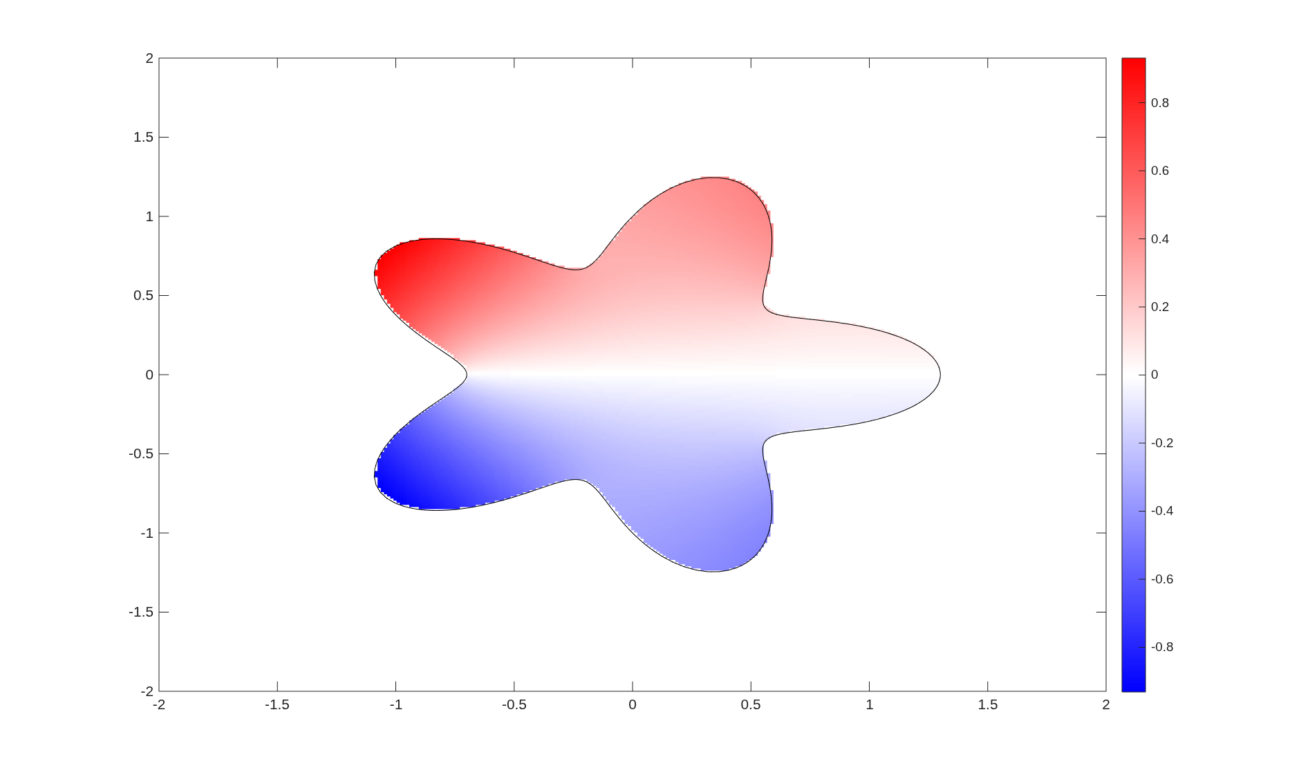
A Laplace Problem

Consider the Laplace Neumann boundary value problem:

\[\begin{split}\begin{aligned} \Delta u &= 0 & \textrm{ in } \Omega \; ,\\ \frac{\partial u}{\partial n} &= f & \textrm{ on } \Gamma \; , \end{aligned}\end{split}\]

where \(n\) is the outward normal. This is a model for the equilibrium heat distribution in a homogeneous medium, where \(f\) is a prescribed heat flux along the boundary.

For a solution to exist, \(f\) must satisfy the compatibility condition:

\[\int_\Gamma f(y) \, ds(y) = 0 \; ,\]

which is equivalent to requiring that there is no net flux of heat into the body. When solutions exist, they are not unique because adding a constant to any solution gives another solution.

The solution of this problem by layer potentials has been well understood for some time. The standard method is reviewed here with a fair amount of detail. Users familiar with the approach may simply want to skip down to the code example.

The Green function for the Laplace equation is

\[G_0 (x,y) = -\frac{1}{2\pi} \log |x-y|\]

The standard choice for the layer potential for this problem is the single layer potential

\[u(x) = [S\sigma](x) := \int_\Gamma G_0(x,y) \sigma(y) ds(y) \; .\]

Then, imposing the boundary conditions on this representation results in the equation

\[\begin{split}\begin{aligned} f(x_0) &= \lim_{x\in \Omega, x\to x_0} n(x_0)\cdot \nabla_x \int_\Gamma G_0(x,y) \sigma(y) \, ds(y) \\ &= \frac{1}{2} \sigma(x_0) + P.V. \int_\Gamma n(x_0) \cdot \nabla_x G_0(x_0,y) \sigma(y) \, ds(y) \\ &=: \left [\left ( \frac{1}{2} \mathcal{I} + \mathcal{S}' \right ) \sigma \right ] (x_0) \; , \end{aligned}\end{split}\]

where \(P.V.\) indicates that the integral should be interpreted in the principal value sense, \(\mathcal{I}\) is the identity operator, and the calligraphic letters indicate that these operators act on functions defined on \(\Gamma\). The second equality above uses a so-called “jump condition” for the single layer potential.

It turns out that the equation for \(\sigma\) above is a second-kind integral equation, i.e. of the form “identity plus compact”, but it is not invertible. This has a simple remedy. The equation

\[f = \left ( \frac{1}{2} \mathcal{I} + \mathcal{S}' + \mathcal{W} \right) \sigma \; ,\]

where

\[[\mathcal{W}\sigma](x) = \int_\Gamma \sigma (y) \, ds(y) \; ,\]

has the same solutions as the original equation (so long as \(f\) satisfies the compatibility condition) and is invertible. The operator \(\mathcal{W}\) is straightforward to discretize:

\[\begin{split}W = \begin{bmatrix} 1 \\ 1 \\ \vdots \\ 1 \end{bmatrix} \begin{bmatrix} w_1 & w_2 & \cdots & w_n \end{bmatrix} \; ,\end{split}\]

where \(w_1,\ldots,w_n\) are scaled integration weights on \(\Gamma\). For historical reasons, the routine that returns this matrix in chunkie is called onesmat.

To discretize the boundary integral equation, chunkie requires a chunker class object discretization of the boundary and a kernel class object representing the integral kernel. Many of the most common kernel types are available in chunkie, including the normal derivative of the single layer kernel, which is called “sprime”. This can be obtained via

kernsp = kernel('lap','sprime');

The most essential thing that an instance of the kernel class tells chunkie is how to evaluate the kernel function. This is stored in the field obj.eval. The object can also store other information about the kernel, such as fast algorithms for its evaluation or the type of singularity it has.

Note

The obj.eval function in a kernel is expected to be of the form eval(s,t), where s and t are structs that specify information about the “sources” and “targets” for which the kernel is being evaluated. This has the unfortunate feature that \(x\) and \(y\) take the roles of “target” and “source”, respectively, in the math notation above, so the order is reversed.

The structs s and t must have the fields s.r and t.r which specify the locations of the sources and targets, respectively. For sources/targets on a chunker object, these will also contain fields s.d, s.d2, s.n, and s.data (likewise for t) containing the chunk information for the corresponding points. For example, the kernel kernsp defined above is only defined for targets on a chunker discretization of a curve and the kernel evaluator kernsp.eval assumes that the field t.n is populated with the normal vectors at the targets.

Because these standard kernels are built into chunkie, this PDE can be solved with very little coding:

% get a chunker discretization of a starfish domain
chnkr = chunkerfunc(@(t) starfish(t));

% define a boundary condition. because of the symmetries of the 
% starfish, this function integrates to zero
pwfun = @(r) r(1,:).^2.*r(2,:);
rhs = pwfun(chnkr.r); rhs = rhs(:);

% get the kernel 
kernsp = kernel('lap','sprime');

% get a matrix discretization of the boundary integral equation 
sysmat = chunkermat(chnkr,kernsp); % just the sprime part
% add the identity term and "ones matrix"
sysmat = sysmat + 0.5*eye(chnkr.npt) + onesmat(chnkr); 

% solve the system 
sigma = gmres(sysmat,rhs);

% grid for plotting solution
x1 = linspace(-2,2,300);
[xx,yy] = meshgrid(x1,x1);
targs = [xx(:).'; yy(:).'];
in = chunkerinterior(chnkr,targs);
uu = nan(size(xx));

% need the single layer, not it's dervative, to evaluate u
kerns = kernel('lap','s');
uu(in) = chunkerkerneval(chnkr,kerns,sigma,targs(:,in));

% plot
figure(1); clf
h = pcolor(xx,yy,uu); set(h,'EdgeColor','none'); colorbar
hold on; plot(chnkr,'k'); colormap(redblue)

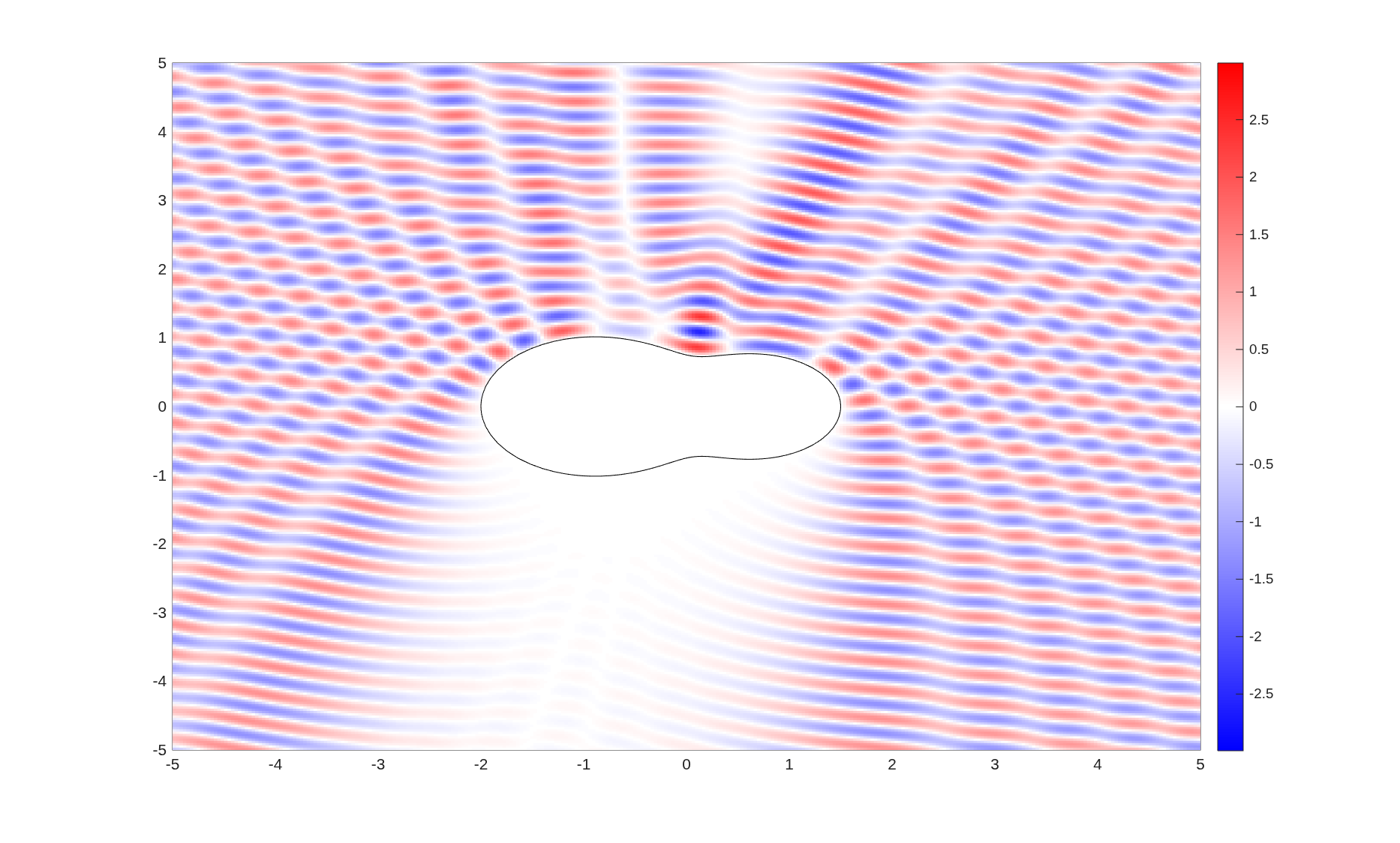
A Helmholtz Scattering Problem

In a scattering problem, an incident field \(u^{\textrm{inc}}\) is specified in the exterior of an object and a scattered field \(u^{\textrm{scat}}\) is determined so that the total field \(u = u^{\textrm{inc}}+u^{\textrm{scat}}\) satisfies the PDE and a given boundary condition. It is also required that the scattered field radiates outward from the object. For a sound-soft object in acoustic scattering, the total field is zero on the object boundary. This results in the following boundary value problem for \(u^{\textrm{scat}}\) in the exterior of the object:

\[\begin{split}\begin{aligned} (\Delta + k^2) u^{\textrm{scat}} &= 0 & \textrm{ in } \mathbb{R}^2 \setminus \Omega \; , \\ u^{\textrm{scat}} &= -u^{\textrm{inc}} & \textrm{ on } \Gamma \; , \\ \sqrt{|x|} \left( \frac{x}{|x|} \cdot \nabla u^{\textrm{scat}} - ik u^{\textrm{scat}} \right ) &\to 0 & \textrm{ as } |x|\to \infty \; , \end{aligned}\end{split}\]

The Green function for the Helmholtz equation is

\[G_k (x,y) = \frac{i}{4} H_0^{(1)}( k|x-y|) \; .\]

Analogous to the above, this Green function can be used to define single and double layer potential operators

\[\begin{split}\begin{aligned} [S\sigma](x) &:= \int_\Gamma G_k(x,y) \sigma(y) ds(y) \\ [D\sigma](x) &:= \int_\Gamma n(y)\cdot \nabla_y G_k(x,y) \sigma(y) ds(y) \end{aligned}\end{split}\]

A robust choice for the layer potential representation for this problem is a combined field layer potential, which is a linear combination of the single and double layer potentials:

\[u^{\textrm{scat}}(x) = [(D - ik S)\sigma](x) \; .\]

Then, imposing the boundary conditions on this representation results in the equation

\[\begin{split}\begin{aligned} -u^{\textrm{inc}}(x_0) &= \lim_{x\in \mathbb{R}^2\setminus \Omega, x\to x_0} [(D-ik S)\sigma](x) \\ &= \frac{1}{2} \sigma(x_0) + [ (\mathcal{D} -ik \mathcal{S})\sigma ](x_0) \end{aligned}\end{split}\]

where we have used the exterior jump condition for the double layer potential. As above, the integrals in the operators restricted to the boundary must sometimes be interpreted in the principal value or Hadamard finite-part sense. The above is a second kind integral equation and is invertible.

As before, this is relatively straightforward to implement in chunkie using the built-in kernels:

% get a chunker discretization of a peanut-shaped domain
modes = [1.25,-0.25,0,0.5];
ctr = [0;0];
chnkr = chunkerfunc(@(t) chnk.curves.bymode(t,modes,ctr));

% the boundary condition is determined by an incident plane wave
kwav = 3*[-1,-5];
pwfun = @(r) exp(1i*kwav*r(:,:));
rhs = -pwfun(chnkr.r); rhs = rhs(:);

% define the CFIE kernel D - ik S
zk = norm(kwav);
coefs = [1,-1i*zk];
kerncfie = kernel('h','c',zk,coefs);

% get a matrix discretization of the boundary integral equation 
sysmat = chunkermat(chnkr,kerncfie); 
% add the identity term
sysmat = sysmat + 0.5*eye(chnkr.npt);

% solve the system 
sigma = gmres(sysmat,rhs,[],1e-10,100);

% grid for plotting solution (in exterior)
x1 = linspace(-5,5,300);
[xx,yy] = meshgrid(x1,x1);
targs = [xx(:).'; yy(:).'];
in = chunkerinterior(chnkr,{x1,x1});
uu = nan(size(xx));

% same kernel to evaluate as on boundary
uu(~in) = chunkerkerneval(chnkr,kerncfie,sigma,targs(:,~in));
uu(~in) = uu(~in) + pwfun(targs(:,~in)).';

% plot
figure(1); clf
h = pcolor(xx,yy,real(uu)); set(h,'EdgeColor','none'); colorbar
colormap(redblue); umax = max(abs(uu(:))); clim([-umax,umax]);
hold on 
plot(chnkr,'k')

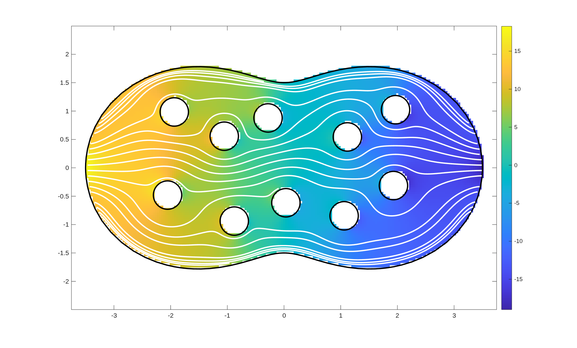
A Stokes Flow Problem

Below, we show a chunkIE solution of a Stokes flow problem in a multiply connected domain. This uses a combined layer representation for Stokes, \(u = (D-S)[\sigma]\) which results in the boundary integral equation

\[f(x_0) = \left [\left ( -\frac{1}{2} \mathcal{I} + \mathcal{D} - \mathcal{S} \right ) \sigma \right ] (x_0) \; ,\]

where \(f\) is a prescribed velocity on the boundary. This equation also has a nullspace, so we add the operator

\[\mathcal{W}\sigma (x) = \int_{\Gamma} n(x) (n(y)\cdot \sigma(y)) \, ds(y)\]

The data \(f\) must have that its normal component integrates to zero. In that case, the equation

\[f(x_0) = \left [\left ( -\frac{1}{2} \mathcal{I} + \mathcal{W} + \mathcal{D} - \mathcal{S} \right ) \sigma \right ] (x_0) \; ,\]

% get a chunker discretization of a peanut-shaped domain
modes = [2.5,0,0,1];
ctr = [0;0];
chnkrouter = chunkerfunc(@(t) chnk.curves.bymode(t,modes,ctr));

% inner boundaries are circles (reverse them to get orientations right)
chnkrcirc = chunkerfunc(@(t) chnk.curves.bymode(t,0.25,[0;0]));
chnkrcirc = reverse(chnkrcirc);
centers = [ [-2:2, -2:2]; [(0.7 + 0.2*(-1).^(-2:2)) , ...
    (-0.7 + 0.2*(-1).^(-2:2))]];
centers = centers + 0.1*randn(size(centers));

% make a boundary out of the outer boundary and several shifted circles
chnkrlist = [chnkrouter];
for j = 1:size(centers,2)
    chnkr1 = chnkrcirc;
    chnkr1 = chnkr1.move([0;0],centers(:,j));
    chnkrlist = [chnkrlist chnkr1];
end
chnkr = merge(chnkrlist);

%%

% boundary condition specifies the velocity. two values per node
wid = 0.3; % determines width of Gaussian
f = @(r) [exp(-r(2,:).^2/(2*wid^2)); zeros(size(r(2,:)))];
rhsout = f(chnkrouter.r(:,:)); rhsout = rhsout(:);
rhs = [rhsout; zeros(2*10*chnkrcirc.npt,1)];

% define the combined layer Stokes representation kernel
c = -1; % coefficient of S
mu = 1; % stokes viscosity parameter
kerncvel = kernel('stok','dvel',mu) + c*kernel('stok','svel',mu);

% get a matrix discretization of the boundary integral equation 
cmat = chunkermat(chnkr,kerncvel); 

% add the identity term and nullspace correction
W = normonesmat(chnkr);
sysmat = cmat - 0.5*eye(2*chnkr.npt) + W;

% solve the system 
sigma = gmres(sysmat,rhs,[],1e-10,100);

% grid for plotting solution (in exterior)
x1 = linspace(-3.75,3.75,200);
y1 = linspace(-2,2,100);
[xx,yy] = meshgrid(x1,y1);
targs = [xx(:).'; yy(:).'];
in = chunkerinterior(chnkr,{x1,y1});
uu = nan([2,size(xx)]);
pres = nan(size(xx));

% same kernel to evaluate as on boundary
uu(:,in) = reshape(chunkerkerneval(chnkr,kerncvel,sigma,targs(:,in)),2,nnz(in));

% can evaluate the associated pressure
kerncpres = kernel('stok','dpres',mu) + c*kernel('stok','spres',mu);
opts = []; opts.eps = 1e-3;
pres(in) = chunkerkerneval(chnkr,kerncpres,sigma,targs(:,in),opts);

% plot
figure(1); clf
h = pcolor(xx,yy,pres); set(h,'EdgeColor','none'); colorbar
colormap("parula");
hold on
plot(chnkr,'k','LineWidth',2); axis equal

figure(1)
u = reshape(uu(1,:,:),size(xx)); v = reshape(uu(2,:,:),size(xx));
startt = linspace(pi-pi/12,pi+pi/12,20);
startr = 0.99*chnk.curves.bymode(startt,modes,[0;0]);
startx = startr(1,:); starty = startr(2,:);

sl = streamline(xx,yy,u,v,startx,starty);
set(sl,'LineWidth',2,'Color','w')

References

[Rok1985]

Rokhlin, Vladimir. “Rapid solution of integral equations of classical potential theory.” Journal of Computational Physics 60.2 (1985): 187-207.

[Poz1992]

Pozrikidis, Constantine. Boundary integral and singularity methods for linearized viscous flow. Cambridge University Press, 1992.

[GL1996]

Guenther, Ronald B., and John W. Lee. Partial differential equations of mathematical physics and integral equations. Courier Corporation, 1996.

[CK2013]

Colton, David, and Rainer Kress. Integral equation methods in scattering theory. Society for Industrial and Applied Mathematics, 2013.

[BGR2010]

Bremer, James, Zydrunas Gimbutas, and Vladimir Rokhlin. “A nonlinear optimization procedure for generalized Gaussian quadratures.” SIAM Journal on Scientific Computing 32.4 (2010): 1761-1788.