Curve Discretization with Chunkers

In chunkie, a smooth, regular curve is discretized by dividing it into pieces, called “chunks”, which are then represented by polynomial interpolants at scaled Legendre nodes. This information is stored in a chunker object.

Creating a Chunker

A chunker object can be obtained from a curve parameterization using the function chunkerfunc. The chunker class overloads some MATLAB commands, like plot and quiver, to simplify common visualization tasks. The code below creates a chunker object for a circle and plots the geometry and the normal vectors.

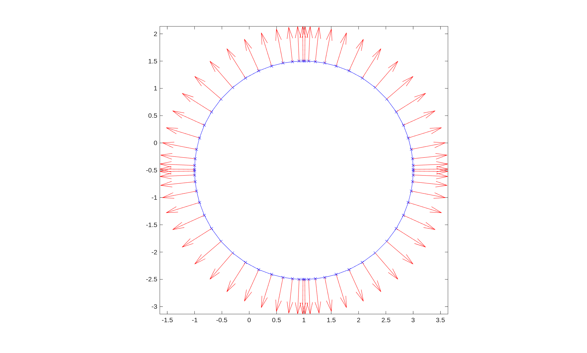
% chunk up circle

rad = 2; ctr = [1.0;-0.5];
circfun = @(t) ctr + rad*[cos(t(:).');sin(t(:).')];

chnkr1 = chunkerfunc(circfun);

% plot curve, nodes, and normals

figure(1)
clf
plot(chnkr1,'b-x')
hold on
quiver(chnkr1,'r')
axis equal tight

Note

The chunkerfunc routine expects a specific format for the curve parameterization function. In particular, if fcurve is a MATLAB function defining the curve parameterization and t is a vector of points in parameter space, then r = fcurve(t) should be a matrix in which r(:,j) contains the \((x,y)\) coordinates of the point on the curve corresponding t(j).

If the output of fcurve is of the form [r,d] = fcurve(t) or [r,d,d2] = fcurve(t), then d and d2 are assumed to be first and second derivatives, respectively, of the position with respect to the underlying parameterization. Providing these values can improve the convergence rate and precision achieved in integral equation calculations.

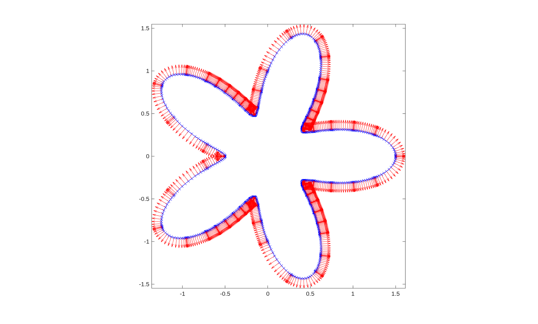
Some utilities are provided that define a family of parameterized curves:

% curvebymode lets you specify a star shaped domain by 
% a cosine/sine series for the radius

modes = randn(11,1); modes(1) = 1.1*sum(abs(modes(2:end))); 
ctr = [1.0;-0.5];
chnkr2 = chunkerfunc(@(t) chnk.curves.bymode(t,modes,ctr));

figure(2)
clf
plot(chnkr2,'b-x')
hold on
quiver(chnkr2,'r')
axis equal tight

% classic starfish domain

narms = 5; 
amp = 0.5;
chnkr3 = chunkerfunc(@(t) starfish(t,narms,amp));

figure(3)
clf
plot(chnkr3,'b-x')
hold on
quiver(chnkr3,'r')
axis equal tight

For a given set of points, a spline curve can be fit to them and discretized as a chunker using chunkerfit:

% Sample a smooth curve at random points
rng(0)
n = 20;
tt = sort(2*pi*rand(n,1));
r = chnk.curves.bymode(tt, [2 0.5 0.2 0.7]);

% can pass cparams and pref structures, as in
% chunkerfunc, via the opts structure
% asking for splitting can be more efficient, dependent on
% desired tolerance

% first asking for lower precision from chunkerfunc
opts = [];
opts.ifclosed = true;
opts.cparams = [];
opts.cparams.eps = 1e-3;
opts.pref = [];
opts.pref.k = 16;
chnkr = chunkerfit(r, opts);

% automatically creates a chunker between each node
opts.splitatpoints = true;
chnkrsp = chunkerfit(r, opts);

% then asking for more precision from chunkerfunc
opts.cparams.eps = 1e-9;
opts.splitatpoints = false;
chnkr2 = chunkerfit(r, opts);

% automatically creates a chunker between each node
opts.splitatpoints = true;
chnkrsp2 = chunkerfit(r, opts);

figure(7)
clf
tiledlayout(2,2,"TileSpacing","compact");
nexttile; plot(chnkr,'k-x'); title(sprintf("nch = %d, eps=1e-3",chnkr.nch));
hold on; plot(r(1,:),r(2,:),'bd');
nexttile; plot(chnkrsp,'k-x'); title(sprintf("nch = %d, eps=1e-3\n (splitting)",chnkrsp.nch));
hold on; plot(r(1,:),r(2,:),'bd');
nexttile; plot(chnkr2,'k-x'); title(sprintf("nch = %d, eps=1e-9",chnkr2.nch));
hold on; plot(r(1,:),r(2,:),'bd');
nexttile; plot(chnkrsp2,'k-x'); title(sprintf("nch = %d, eps=1e-9\n (splitting)",chnkrsp2.nch));
hold on; plot(r(1,:),r(2,:),'bd');

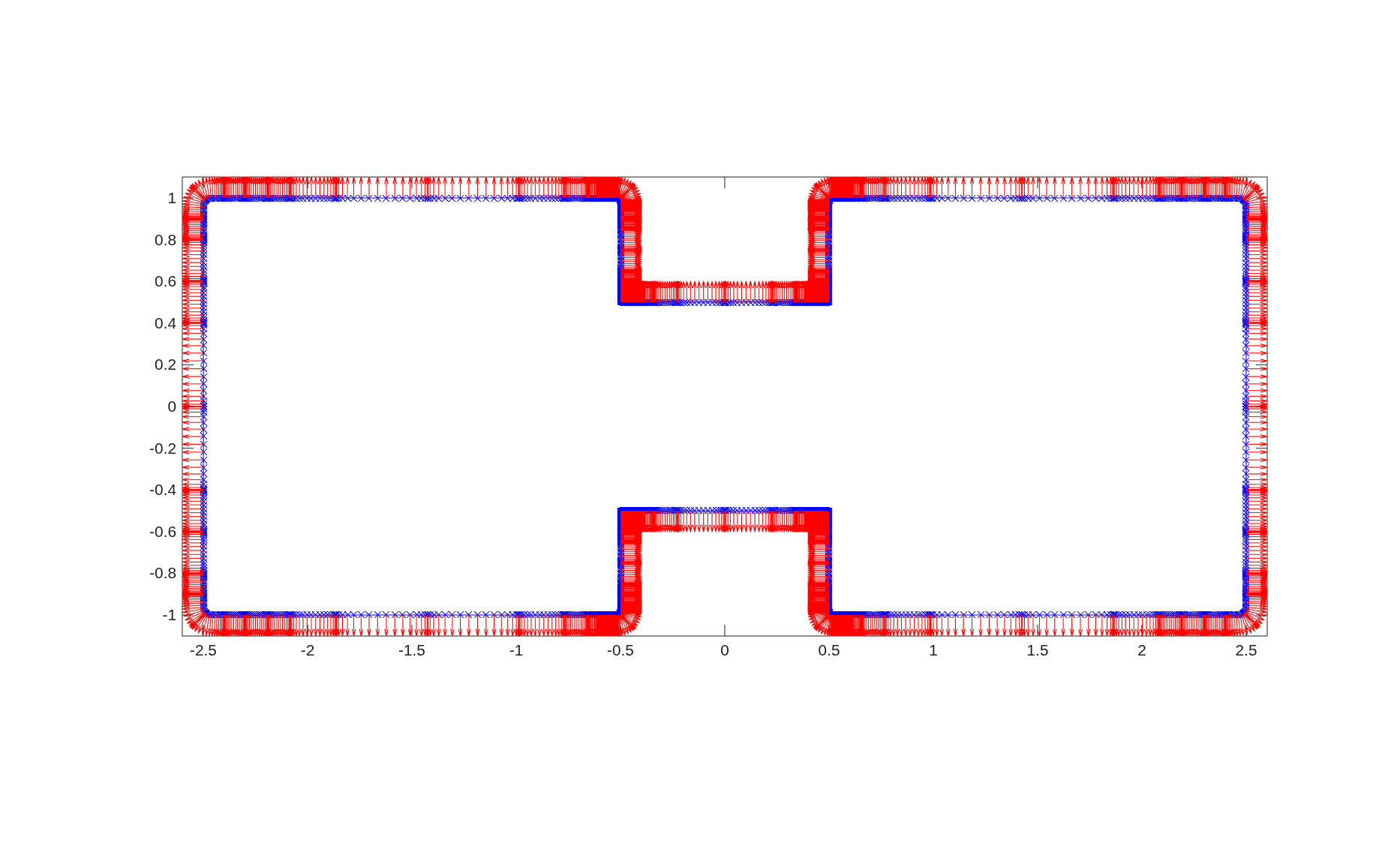
Given a set of vertices, a rounded polygon can be defined:

% chunkerpoly provides a chunk discretization of a rounded polygon

verts = chnk.demo.barbell(2.0,2.0,1.0,1.0); % vertices of a barbell
chnkr4 = chunkerpoly(verts);

figure(4)
clf
plot(chnkr4,'b-x')
hold on
quiver(chnkr4,'r')
axis equal tight

Working with Chunkers

Instances of chunker objects can be manipulated in several ways. Multiplying the object by a matrix and adding a vector to the object will update the coordinates (and derivatives and normals) accordingly. There are also some built in functions for standard operations like rotations and reflections. An important operation is the reverse function, which changes the orientation of the curve (normal vectors point to the right from the perspective of an observer moving in the positive direction along the curve).

The example below takes the circle and random mode domains created above and creates a new domain from them with multiple components. The random mode domain is rotated and reflected, then its orientation is reversed to undo the change of orientation induced by the reflection (maintaining outward pointing normals). An affine transformation is applied to the circle and its orientation is also reversed, so that the normal for the combined domain consistently points out of the interior.

% make a copy of the random mode domain
chnkr5 = chnkr2;

% rotate it using rotate method
theta = pi/4; 
chnkr5 = chnkr5.rotate(theta);

% reflect it across y axis using reflect
chnkr5 = chnkr5.reflect(pi/2);
% reverse orientation to get inward normals again (reflect changes
% orientation)
chnkr5 = chnkr5.reverse();

% make a copy of the circle domain, transform and shift it 
chnkr6 = chnkr1;
A = 0.5*[2 -1; 1 1]; % positive determinant, so doesn't change orientation
r1 = [-1;0.5];
chnkr6 = r1 + A*chnkr6;
% reverse the orientation
chnkr6 = chnkr6.reverse();

% merge these two curves into one domain
chnkr7 = merge([chnkr5,chnkr6]);

figure(5); clf
plot(chnkr7,'b-x'); hold on; quiver(chnkr7,'r')
axis equal tight

It is also possible to find the points on the interior of a chunker object, which is convenient in many plotting tasks:

% create a grid of points 
mins = min(chnkr7); maxs = max(chnkr7);
x1 = linspace(mins(1),maxs(1)); y1 = linspace(mins(2),maxs(2));
[xx,yy] = meshgrid(x1,y1);
pts = [xx(:).'; yy(:).'];

% find the points inside the merged domain
in = chunkerinterior(chnkr7,pts);

zz = nan(size(xx));
zz(in) = 1;

figure(6)
h = pcolor(xx,yy,zz); set(h,'EdgeColor','none');
axis equal tight

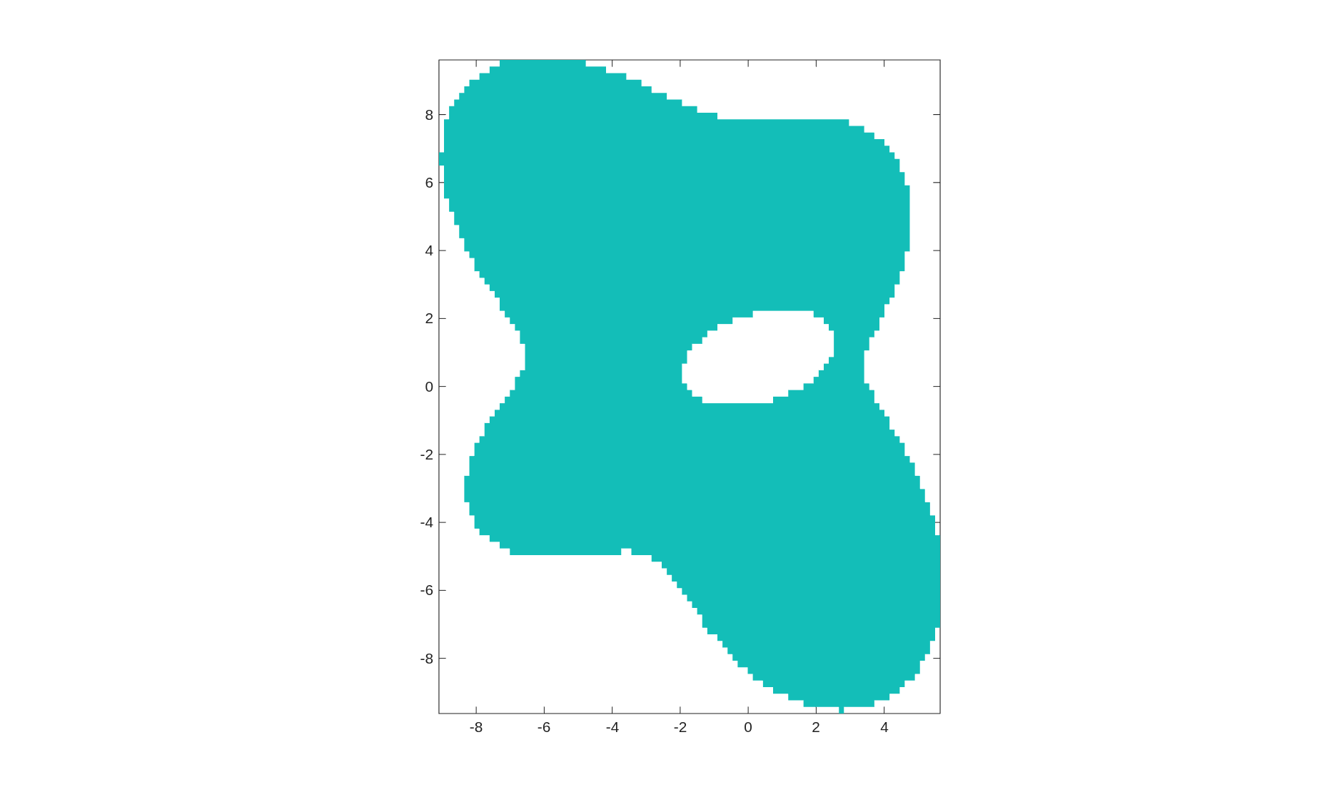
Note

In the example above, it is crucial that the orientation of the circle was reversed so that the combined domain had consistent normals, i.e. so that the normals all pointed out of the interior. Without doing this, the chunkerinterior function will fail.

There is more available. The chunker class documentation gives a survey of the available methods:

%CHUNKER class which describes a curve divided into chunks (or "panels"). 
%
% On each chunk the curve is represented by the values of its position, 
% first and second derivatives by scaled Legendre nodes.
%
% chunker properties:
%   k - integer, number of Legendre nodes on each chunk
%   nch - integer, number of chunks that make up the curve
%   dim - integer, dimension of the ambient space in which the curve is 
%             embedded
%   npt - returns k*nch, the total number of points on the curve
%   r - dim x k x nch array, r(:,i,j) gives the coordinates of the ith 
%         node on the jth chunk of the chunker
%   d - dim x k x nch array, d(:,i,j) gives the time derivative of the 
%         coordinate at the ith node on the jth chunk of the chunker
%   d2 - dim x k x nch array, d(:,i,j) gives the 2nd time derivative of the 
%         coordinate at the ith node on the jth chunk of the chunker
%   n - dim x k x nch array of normals to the curve
%   data - datadim x k x nch array of data attached to chunker points 
%         this data will be refined along with the chunker
%   adj - 2 x nch integer array. adj(1,j) is i.d. of the chunk that 
%         precedes chunk j in parameter space. adj(2,j) is the i.d. of the
%         chunk which follows. if adj(i,j) is 0 then that end of the chunk
%         is a free end. if adj(i,j) is negative than that end of the chunk
%         meets with other chunk ends in a vertex. the specific negative
%         number acts as an i.d. of that vertex.
%
% chunker methods: 
%   chunker(p,t,w) - construct an empty chunker with given preferences and
%       precomputed Legendre nodes/weights (optional)
%   obj = plus(v,obj) - provides translation via v + obj
%   obj = mtimes(A,obj) - provides affine transformation via A*obj
%   obj = rotate(obj,theta,r0,r1) - rotate by angle 
%   obj = reflect(obj,theta,r0,r1) - reflect across line
%   obj = addchunk(obj,nchadd) - add nchadd chunks to the structure 
%       (initialized with zeros)
%   obj = makedatarows(obj,nrows) - add nrows rows to the data storage.
%   [obj,info] = sort(obj) - sort the chunks so that adjacent chunks are
%        stored sequentially
%   [rn,dn,d2n,dist,tn,ichn] = nearest(obj,ref,ich,opts,u,xover,aover) -
%        find nearest point on chunker to ref
%   obj = reverse(obj) - reverse chunk orientation
%   rmin = min(obj) - minimum of coordinate values
%   rmax = max(obj) - maximum of coordinate values
%   wts = weights(obj) - scaled integration weights on curve
%   obj.n = normals(obj) - recompute normal vectors
%   onesmat = onesmat(obj) - matrix that corresponds to integration of a
%             density on the curve
%   rnormonesmat = normonesmat(obj) - matrix that corresponds to
%             integration of dot product of normal with vector density on
%             the curve
%   plot(obj,varargin) - plot the chunker curve
%   plot3(obj,idata,varargin) - 3D plot of the curve and one row of the
%             data storage
%   quiver(obj,varargin) - quiver plot of the chnkr points and normals
%   scatter(obj,varargin) - scatter plot of the chnkr nodes
%   tau = taus(obj) - unit tangents to curve
%   cgrph = tochunkgraph(obj) - convert to chunkgraph
%   obj = refine(obj,varargin) - refine the curve
%   a = area(obj) - for a closed curve, area inside 
%   s = arclength(obj) - get values of arclength along curve
%   kappa = signed_curvature(obj) - get signed curvature along curve
%   rflag = datares(obj,opts) - check if data in data rows is resolved
%   [rc,dc,d2c] = exps(obj) - get expansion coefficients for r,d,d2
%   ier = checkadjinfo(obj) - checks that the adjacency info of the curve
%              is consistent
%   [inds,adjs,info] = sortinfo(obj) - attempts to sort the curve and finds
%              number of connected components, etc
%   [re,taue] = chunkends(obj,ich) - get the endpoints of chunks
%   flag = flagnear(obj,pts,opts) - flag points near the boundary
%   obj = obj.move(r0,r1,trotat,scale) - translate, rotate, etc

Note

To obtain the documentation of a class method which has overloaded the name of a MATLAB built-in, use the syntax help class_name/method_name. For example:

help chunker/area