Describing More Complicated Geometries with Chunkgraphs

Many practical applications, especially those involving corners and multiple junction interfaces, require a more detailed description of the geometry, beyond an array of chunker objects. While it is relatively easy to specify these more complicated problems, integral equation methods require special care in the vicinity of corners and mutltiple junctions in order to achieve high precision. The requisite additional information can be stored in chunkie in a chunkgraph object, which is essentially a collection of chunker objects and a graph-theoretic description of their connectivity. In particular, each smooth boundary component, stored as a chunker, corresponds to an edge of the graph, and points where multiple smooth boundary components meet (or where a smooth component ends), correspond to vertices of the graph.

Creating Chunkgraphs

The easiest way to define chunkgraphs is using its constructor which requires at least two inputs, a collection of vertices and connectivity information specified as a (2,nedges) array with each column corresponding to the indices of the vertices defining the edge. The edge is directed and begins at the vertex in the first row and ends at the vertex in the corresponding second row.

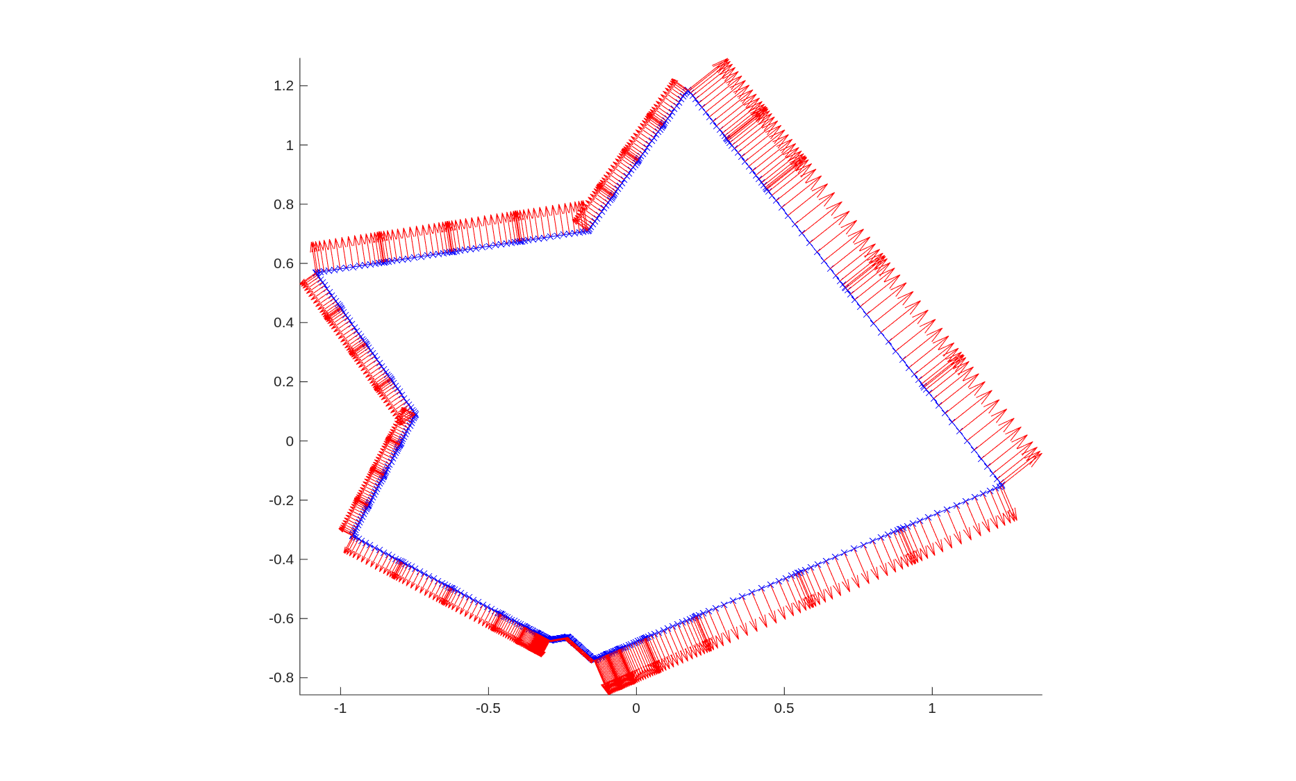
In the example below, we construct a polygon defined as a chunkgraph. As before we can visualize the chunkgraph using overloaded MATLAB commands plot and quiver.

% chunk up random polygon

rng(123)
t = sort(2*pi*rand(9,1));
verts = starfish(t,5,0.3);
[~, nv] = size(verts);
edgesendverts = [1:nv; circshift(1:nv,-1)];
cgrph1 = chunkgraph(verts, edgesendverts);

% plot curve, nodes, and normals

figure(1)
clf
plot(cgrph1,'b-x')
hold on
quiver(cgrph1,'r')
axis equal tight

Instead of having straight edges, the user can define curved edges between vertices as well. This is specified either as a single function handle, in which case all edges would be defined by the same function handle, or via a cell array of function handles, where vertices are connected by a straight edge if the corresponding element of the cell array of function handles is empty. Each function handle must have the same specification as the ones used to define chunkers, i.e., if fcurve is a MATLAB function defining the curve parametrization and t is a vector fo points in parameter space, then the output of fcurve is of the form [r] = fcurve(t) or [r,d] = fcurve(t) or [r,d,d2] = fcurve(t) where r are the coordinates of the points on the curve, d is the first derivative of the position with respect to the underlying parametrization and d2 is the corresponding second derivative. For ease of specification, the curves described by the function handles aren’t required to terminate exactly at the appropriate vertices; the chunkgraph constructor will snap the edge to its vertices via an appropriate affine transformation.

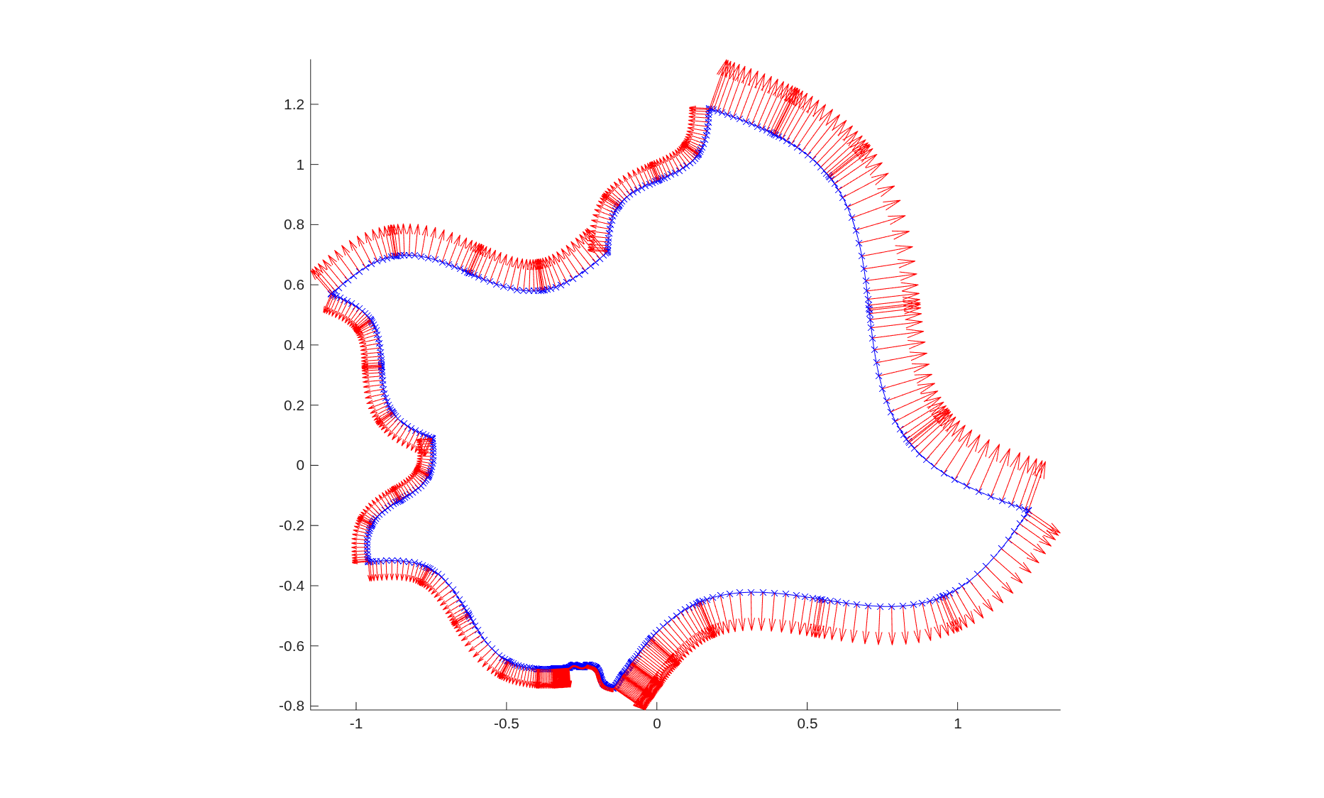
Here is an example illustrating a square whose edges are defined via a sine wave.

% Make all edges of the above chunkgraph curved


fcurve = @(t) chnk.curves.fsine(t,0.1,2*pi,0);
cgrph2 = chunkgraph(verts, edgesendverts, fcurve);


figure(2)
clf
plot(cgrph2,'b-x')
hold on
quiver(cgrph2,'r')
axis equal tight

Note

The default domain of parameter space defining an edge of a chunkgraph is [0,1] as opposed to that of a chunker which is [0,2pi).

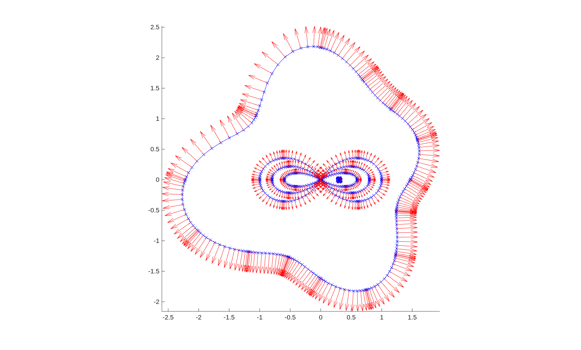
The same constructor interface is capable of creating complicated domains including ones with loops starting and ending at the same vertex, multiple junctions, and nested regions. The constructor is also capable of handling chunkgraphs with smooth closed curves which are treated as edges with no vertices. All of these are illustrated in the construction of the complicated hawaiian earing with a nested star-fish below.

verts =[0;0];
funcs = cell(8,1);
funcs{1} = @(t) hawaiian(t,pi/3,0.6);
funcs{2} = @(t) hawaiian(t,pi/3,-0.6);
funcs{3} = @(t) hawaiian(t,pi/4,0.8);
funcs{4} = @(t) hawaiian(t,pi/4,-0.8);
funcs{5} = @(t) hawaiian(t,pi/6,1);
funcs{6} = @(t) hawaiian(t,pi/6,-1);

rng(1);
modes1 = 0.002*randn(11,1); modes1(1) = 0.03; 
ctr1 = [0.3;0];

modes2 = 0.1*randn(11,1); modes2(1) = 1.75; 
ctr2 = [0;0];

funcs{7} = @(t) chnk.curves.bymode(t, modes1, ctr1);
funcs{8} = @(t) chnk.curves.bymode(t, modes2, ctr2);

edgesendverts = ones(2,8);
edgesendverts(:,7:8) = nan;

cparams_closed = []; cparams_closed.ta = 0; cparams_closed.tb = 2*pi;
cparams = cell(8,1);
cparams{7} = cparams_closed;
cparams{8} = cparams_closed;
cgrph3 = chunkgraph(verts, edgesendverts, funcs, cparams);

figure(3)
clf
plot(cgrph3,'b-x')
hold on
quiver(cgrph3,'r')
axis equal tight

Working with chunkgraphs

Most functions overloaded for chunkers also work with chunkgraphs. As with chunkers,users are free to edit the position and derivative fields of the chunkgraph objects, or even replace the individual chunkers that define the chunkgraph, and the software will not check if the user has updated the chunkgraph in a consistent manner.

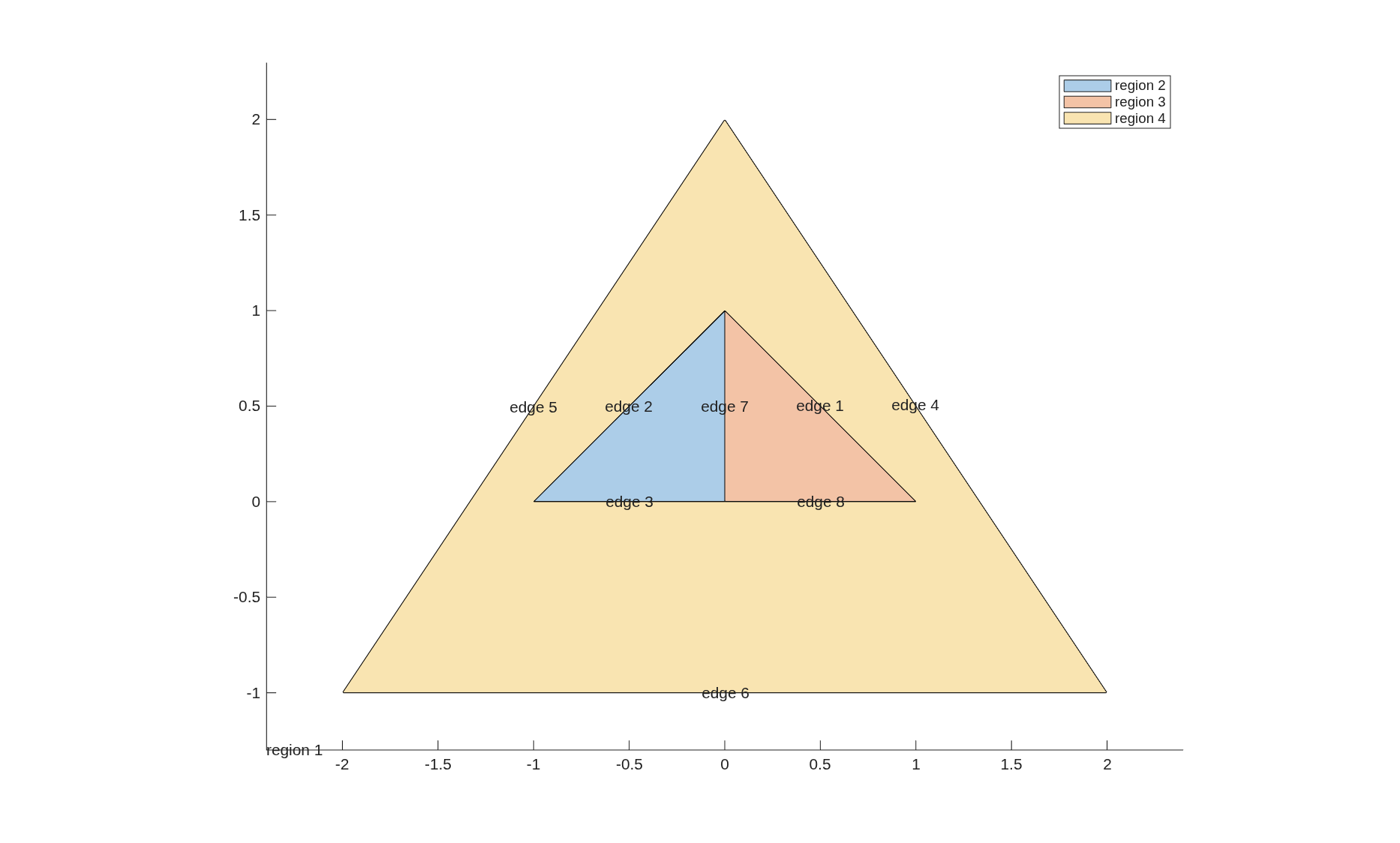
In addition to these routines, we provide an additional plotting routine which labels the edges and regions defined by the chunkgraph. This functionality is illustrated in the example below.

For more details of how this information is stored in the chunkgraph object and to see a survey of other available methods, see the chunkgraph class documentation:

%CHUNKGRAPH class which describes a domain using "graph"
% of chunkers. Singular points of the geometry (or of the
% boundary value problem) are the vertices of the graph. Smooth, regular
% curves are the edges of the graph. The interiors of distinct edges should 
% not intersect. For such domains, a vertex should be introduced at the 
% point of intersection and the curves broken so that they do not intersect.
%
% chunkgraph properties:
%
%   verts - 2 x nverts array of vertex locations 
%   edgesendverts - 2 x nedges array of starting and ending vertices for
%      each edge. edgesendverts(:,i) should be NaNs for closed loops,
%      and a corresponding function handle must be provided
%   echnks - nedge x 1 array of chunker objects discretizing each edge curve
%   regions - nregions x 1 cell array specifying region information for the
%      given graph structure. A region is a connected subset of R^2 
%      specified by its bounding edges. If the jth region is simply 
%      connected then abs(regions{j}{1}) is the list of edges which 
%      comprise the boundary of region j. The sign of the edges indicate
%      the direction of traversal for that edge. The edges are ordered
%      according to an orientation based on nesting. The boundary of the
%      outermost (unbounded) region is traversed clockwise. 
%   vstruc - nverts x 1 cell array. vstruc{j}{1} gives a list of edges which
%      are incident to a vertex. vstruc{j}{2} is a list of the same length
%      consisting of +1 and -1. If +1 then the corresponding edge ends at
%      the vertex, if -1 it begins at the vertex.
%   v2emat - sparse nedge x nverts matrix, akin to a connectivity matrix.
%      the entry v2emat(i,j) is 1 if edge i ends at vertex j, it is -1 if
%      edge i starts at vertex j, and it is 2 if edge i starts and ends at
%      vertex j.
%   k - integer, number of Legendre nodes on each chunk
%   dim - integer, dimension of the ambient space in which the curve is 
%             embedded
%   In the rest, nch = \sum_{j} chunkgraph.echnks(j).nch;
%   npt - returns k*nch, the total number of points on the curve
%   r - dim x k x nch array, r(:,i,j) gives the coordinates of the ith 
%         node on the jth chunk of the chunkgraph
%   d - dim x k x nch array, d(:,i,j) gives the time derivative of the 
%         coordinate at the ith node on the jth chunk of the chunkgraph
%   d2 - dim x k x nch array, d(:,i,j) gives the 2nd time derivative of the 
%         coordinate at the ith node on the jth chunk of the chunkgraph
%   n - dim x k x nch array of normals to the curve
%   data - datadim x k x nch array of data attached to chunkgraph points 
%         this data will be refined along with the chunkgraph
%   adj - 2 x nch integer array. adj(1,j) is i.d. of the chunk that 
%         precedes chunk j in parameter space. adj(2,j) is the i.d. of the
%         chunk which follows. If adj(i,j) is 0 then that end of the chunk
%         is a free end. if adj(i,j) is negative than that end of the chunk
%         meets with other chunk ends in a vertex. 
%
% chunkgraph methods:
%   obj = plus(v,obj) - provides translation via v + obj
%   obj = mtimes(A,obj) - provides affine transformation via A*obj
%   obj = rotate(obj,theta,r0,r1) - rotate by angle 
%   obj = reflect(obj,theta,r0,r1) - reflect across line
%   plot(obj, varargin) - plot the chunkgraph
%   quiver(obj, varargin) - quiver plot of chunkgraph points and normals
%   plot_regions(obj, iflabel) - plot the chunkgraph with region and 
%                  and edge labels
%   scatter(obj,varargin) - scatter plot of the chunkgraph nodes
%   obj = refine(obj,varargin) - refine the curve
%   wts = weights(obj) - scaled integration weights on curve
%   rn = normals(obj) - recompute normal vectors
%   flag = flagnear(obj,pts) - find points close to the chunkgraph
%   flag = flagnear_rectangle(obj,pts) - find points close to chunkgraph
%           using bounding rectangles
%   flag = flagnear_rectangle_grid(obj,x,y) - find points defined via 
%      a meshgrid of points that are close to the chunkgraph
%   rmin = min(obj) - minimum of coordinate values
%   rmax = max(obj) - maximum of coordinate values
%   onesmat = onesmat(obj) - matrix that corresponds to integration of a
%             density on the chunkgraph
%   rnormonesmat = normonesmat(obj) - matrix that corresponds to
%             integration of dot product of normal with vector density on
%             the chunkgraph
%   tau = tangents(obj) - unit tangents to curve
%   kappa = signed_curvature(obj) - get signed curvature along curve
%   obj = makedatarows(obj,nrows) - add nrows rows to the data storage.
%   rflag = datares(obj,opts) - check if data in data rows is resolved
%   edge_reg = find_regions_of_edges(obj) - determine regions on either 
%                side of each edge
%

Note

To obtain the documentation of a class method which has overloaded the name of a MATLAB built-in, use the syntax help class_name/method_name. For example:

help chunkgraph/move