Boundary Value Problems on Chunkgraphs

The solution and behavior of integral equations on chunkgraphs differs from that on chunkers in one major way, the solutions on domains with corners and multiple junctions tend to be singular and require additional care for their accurate computation.

For concreteness, suppose that \(\Gamma\) is the boundary described via a chunkgraph, and consider the following second kind integral equation for a density \(\sigma\)

\[\sigma(x) + \int_{\Gamma} K(x,y) \sigma(y) ds(y) = f(x)\;, \quad x \in \Gamma \,.\]

If \((0,0)\) is a vertex on \(\Gamma\), then for \(x\in \Gamma\) in the vicinity of the corner, \(\sigma\) is well-approximated by functions of the form \(|r|^{\mu} \log{r}^{\eta}\) where \(r=|x|\), \(\mu \in \mathbb{C}\) with \(\textrm{Re}(\mu) > -1\) and \(\eta \in \mathbb{R} \geq 0\). For example, for the Laplace and Helmholtz Neumann boundary value problem, \(\mu \in \mathbb{R} > -1/2\). The approximation of such functions with Gauss-Legendre panel based discretizations to a tolearance of \(\varepsilon\) could require a dyadic grid in the vicinity of the corner with the smallest panel scaling as \(O(1/\varepsilon^2)\).

There are several standard approaches which compress the interactions in the vicinity of the corner with the rest of the boundary. In chunkIE, we use the Recursively compressed inverse preconditioning (RCIP) approach for addressing this issue, since it is robust, capable of achieving high accuracy, kernel indpendent and requires only a quadrature rule for handling the near singular nature of the kernel ignoring the singular behavior of the density. Briefly, it constructs an effective matrix of interaction corresponding to the two panels in the vicinity of the corner, by recursively compressing the corner interactions on a heirarchy of dyadic grids. While a dyadic mesh is used to construct the effective matrix of interaction, the density \(\sigma\) is described by its samples on two Gauss-Legendre panels in the vicinity of the corner. For a detailed description of the RCIP method, see the wonderful tutorial by Johan Helsing who has been the chief architect of the RCIP approach, [Hel2012].

However, the chunkIE user does not have to worry about all of these issues and the routines chunkermat and chunkerkerneval can be seamlessly used for chunkgraphs with only a minor caveat, discussed in the note below.

Note

The integral equation must be appropriately scaled to ensure that it is of the form \((I + K)\) as opposed to \(\alpha I + K\) for \(\alpha \neq 1\). The current implementation of the corner compression scheme, RCIP, requires this scaling for solving integral equations on chunkgraphs. This restriction will soon be lifted in an upcoming release of chunkIE, but is required as of the current version.

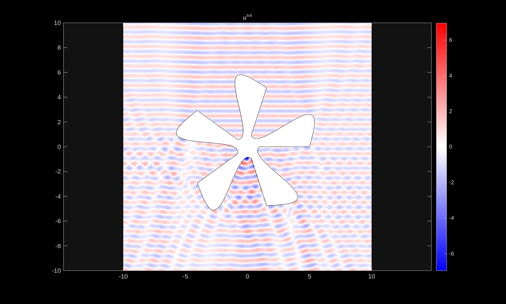
A Sound Hard Scattering Problem with Corners

Consider the Helmholtz Neumann scattering problem in the exterior of a domain with corners. As before, in such a scattering problem, an incident field \(u^{\textrm{inc}}\) is specified in the exterior of the object and the scattered field \(u^{\textrm{scat}}\) is determined so that the total field \(u = u^{\textrm{inc}} + u^{\textrm{scat}}\) satisfies the following PDE:

\[\begin{split}\begin{aligned} (\Delta + k^2) u^{\textrm{scat}} &= 0 & \textrm{ in } \mathbb{R}^2 \setminus \Omega \; , \\ \frac{\partial u^{\textrm{scat}}}{\partial n} &= -\frac{\partial u^{\textrm{inc}}}{\partial n} & \textrm{ on } \Gamma \; , \\ \sqrt{|x|} \left( \frac{x}{|x|} \cdot \nabla u^{\textrm{scat}} - ik u^{\textrm{scat}} \right ) &\to 0 & \textrm{ as } |x|\to \infty \; , \end{aligned}\end{split}\]

The Green function for the Helmholtz equation is

\[G_k (x,y) = \frac{i}{4} H_0^{(1)}( k|x-y|) \; .\]

This Green function can be used to define single and double layer potential operators

\[\begin{split}\begin{aligned} [S_{k}\sigma](x) &:= \int_\Gamma G_k(x,y) \sigma(y) ds(y) \\ [D_{k}\sigma](x) &:= \int_\Gamma n(y)\cdot \nabla_y G_k(x,y) \sigma(y) ds(y) \end{aligned}\end{split}\]

A robust choice for the layer potential representation for this problem is a right preconditioned combined field layer potential, which is a linear combination of the single and double layer potentials:

\[u^{\textrm{scat}}(x) = \beta[(S_{k} + i\alpha D_{k} S_{ik})\sigma](x) \; ,\]

with \(\alpha in \mathbb{R}\) typically chosen to be \(|k|\) and \(\beta = -4.0/(2 + i \alpha)\). See [Bru2009] for a detailed discussion on the benefits of using this particular representation for the Helmholtz Neumann boundary value problem. The seemingly weird scaling of the integral representation is to ensure that the eventual integral equation is of the form \((I+K)\).

Then, imposing the boundary conditions on this representation results in the equation

\[\begin{split}\begin{aligned} -\frac{\partial u^{\textrm{inc}}(x_0)}{\partial n} &= \lim_{x\in \mathbb{R}^2\setminus \Omega, x\to x_0} \beta[(S_{k} + i\alpha D_{k} S_{ik})\sigma](x) \\ &= \sigma(x_0) + \beta[S_{k}'\sigma ](x_0) + i\beta \alpha [(D_{k}' - D_{ik}')S_{ik}\sigma](x_{0}) + i \beta \alpha [S_{ik}'S_{ik}'\sigma](x_0) \;, \end{aligned}\end{split}\]

where \(S_{k}'\) and \(D_{k}'\) represent the normal derivatives of the single and double layer potentials respectively, and we have used the exterior jump condition for \(S_{k}'\) and used Calderon identities to express \(D_{ik}'S_{ik}\) in terms of the identity operator and \(S_{ik}'S_{ik}'\). As before, the integrals in the operators restricted to the boundary must sometimes be interpreted in the principal value or Hadamard finite-part sense. The above is a second kind integral equation and is invertible. The integral equation as written requires operator composition and RCIP in chunkIE does not support such operator compositions. However, this is easily remedied by setting \(-[S_{ik}\sigma](x) + \tau(x) = 0\), and \(-[S_{ik}'\sigma](x) + \mu(x) = 0\) to obtain the following system of equations for \(\sigma, \tau, and \mu\):

\[\begin{split}\begin{bmatrix} \sigma \\ \tau \\ \mu \end{bmatrix} + \begin{bmatrix} \beta S_{k}' & i\beta \alpha (D_{k}'-D_{ik}') & i\beta\alpha S_{ik}' \\ -S_{ik} & 0 & 0 \\ -S_{ik}' & 0 & 0 \end{bmatrix} \begin{bmatrix} \sigma \\ \tau \\ \mu \end{bmatrix} = \begin{bmatrix} -\frac{\partial u^{\textrm{inc}}}{\partial n} \\ 0 \\ 0 \end{bmatrix} \; .\end{split}\]

Recall that the kernel class in chunkIE, also allows for the easy specification of such a matrix of kernels either manually or by reinvoking the constructor on a matrix of objects where each entry of the matrix is a kernel itself.

Thus implementing this problem remains relatively straightforward as illustrated below:

% planewave direction
kvec = [0;8];
zk = norm(kvec);

% make vertices
narms = 5;
rots = exp(1i*2*pi*(1:narms)/narms);
verts = zeros(2,2*narms);
radi = 1;
rado = 5;
for i = 1:narms
    verts(:,2*i-1) = radi*[real(rots(i));imag(rots(i))];
    verts(:,2*i) = rado*[real(rots(i));imag(rots(i))];
end
nverts = size(verts,2);
edge2verts = [1:nverts;circshift(1:nverts,-1)];

% curve parameters
amp = -0.5;
frq = 5;

% define curve for each edge
fchnks = cell(2*narms,1);
for i = 1:narms
    % odd edges are straight
    fchnks{2*i-1} = [];
    % even edges are curved
    fchnks{2*i} = @(t) sinearc(t,amp,frq);
end

cparams = [];
cparams.maxchunklen = min(4.0/zk,.5);
[cgrph] = chunkgraph(verts,edge2verts,fchnks,cparams);

%% Define system

% define kernels
Sk     = kernel('helmholtz', 's', zk);
Skp    = kernel('helmholtz', 'sprime', zk);
Dk     = kernel('helmholtz', 'd', zk);

% combined field uses modified-Helmholtz kernels
Sik    = kernel('helmholtz', 's', 1i*zk);
Sikp   = kernel('helmholtz', 'sprime', 1i*zk);
Dkdiff = kernel('helmdiff', 'dprime', [zk 1i*zk]);

Z = kernel.zeros();

alpha = 1;
c1 = -1/(0.5 + 1i*alpha*0.25);
c2 = -1i*alpha/(0.5 + 1i*alpha*0.25);
c3 = -1;

% define a matrix valued kernel, which corresponds to unpacking the
% composition of operators
K = [ c1*Skp  c2*Dkdiff c2*Sikp ;
   c3*Sik  Z        Z        ;
   c3*Sikp Z        Z        ];
K = kernel(K);


Keval = c1*kernel([Sk 1i*alpha*Dk Z]);

npts = cgrph.npt;
nsys = K.opdims(1)*npts;
start = tic;
A = chunkermat(cgrph, K) + eye(nsys); 
tmat = toc(start)

%% solve system
% Set up boundary data
sources = [4;1];
strengths = 1;

rhs = zeros(nsys,1);
% get Neumann boundary data
rhs_n = -sum(kvec(:).*cgrph.n(:,:),1).*planewave(kvec(:),cgrph.r(:,:));

% only first row of K is physical
rhs(1:K.opdims(1):end) = rhs_n(:);

% solve
start = tic;
sol = gmres(A, rhs, [], 1e-13, 200);
tsolve = toc(start)

%% compute field

L = 2*rado;
x1 = linspace(-L,L,300);
[xx,yy] = meshgrid(x1,x1);
targs = [xx(:).'; yy(:).'];
ntargs = size(targs,2);

% identify points in computational domain
in = chunkerinterior(cgrph,{x1,x1});
out = ~in;

% get incoming solution
uin = nan(size(xx));
uin(out) = planewave(kvec(:),targs(:,out));

% get solution
opts = [];
opts.forcesmooth = false;
uscat = nan(size(xx));
uscat(out) = chunkerkerneval(cgrph,Keval,sol,targs(:,out),opts);

utot = uin + uscat;

%% make plots
umax = max(abs(utot(:))); 
figure(2);clf
h = pcolor(xx,yy,imag(utot)); set(h,'EdgeColor','none'); colorbar
colormap(redblue); clim([-umax,umax]);
hold on 
plot(cgrph,'k')
axis equal
title('$u^{\textrm{tot}}$','Interpreter','latex','FontSize',12)

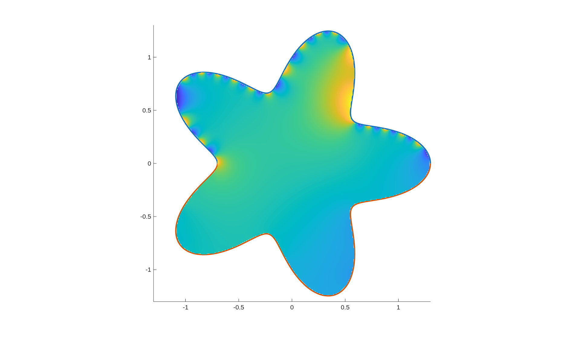
Mixed Boundary Conditions

Singularities arise solutions to PDEs and related integral equations when different parts of the boundary impose different boundary conditions. For simplicity, consider the following Laplace mixed boundary value problem for the potential \(u\) on a domain \(\Omega\) with boundary \(\Gamma\),

\[\begin{split}\begin{aligned} \Delta u &= 0 & \textrm{ in } \Omega \; , \\ u &= f_{D} & \textrm{ on } \Gamma_{D} \; , \\ \frac{\partial u}{\partial n} &= f_{N} & \textrm{ on } \Gamma_{N} \; , \end{aligned}\end{split}\]

where \(\Gamma_{D}\) and \(\Gamma_{N}\) are a partition of the boundary, i.e. \(\Gamma = \Gamma_{D} \cup \Gamma_{N}\), with \(\Gamma_{D} \cup \Gamma_{N} = (0,0)\). Then as above, the solution to the PDE and the associated integral equation is singular in the vicinity of the origin and can be well-approximated by functions of the form \(r^{\mu} \log(r)^{\eta}\) with \(\mu \in \mathbb{R} > -1/2\), and \(\eta \geq 0\). This singular behavior persists even when the boundary is smooth across the origin. Thus, to handle such mixed boundary value problems, it is essential to use chunkgraphs instead of chunkers to define such boundary value problems, with a vertex introduced at every point at which the boundary conditions change.

Recall that the Green function for the Laplace equation is

\[G_0 (x,y) = -\frac{1}{2\pi} \log |x-y|\]

The standard choice for solving such a mixed boundary value problem is to use a single layer potential on \(\Gamma_{N}\) and a double layer potential on \(\Gamma_{D}\),

\[u(x) = 2[S_{\Gamma_{N}}\sigma_{N}](x) - 2[D_{\Gamma_{D}}\sigma_{D}](x)\]

where

\[\begin{split}\begin{aligned} [S_{\Gamma_{N}}\sigma_{N}](x) = \int_{\Gamma_{N}} G_0(x,y) \sigma_{N}(y) ds(y) \; ,\\ [D_{\Gamma_{D}}\sigma_{D}](x) = \int_{\Gamma_{D}} n(y) \cdot \nabla_{y} G_0(x,y) \sigma_{D}(y) ds(y) \; . \end{aligned}\end{split}\]

On imposing the boundary conditions, we get the following system of integral equations for \(\sigma_{D}\) and \(\sigma_{N}\)

\[\begin{split}\begin{aligned} \sigma_{D}(x) - 2[D_{\Gamma_{D}}\sigma_{D}](x) + 2[S_{\Gamma_{N}}\sigma_{N}](x) &= f_{D} \,, \,\, \textrm{ on } \Gamma_{D} \,, \\ \sigma_{N}(x) - 2[D'_{\Gamma_{D}}\sigma_{D}](x) + 2[S'_{\Gamma_{N}}\sigma_{N}](x) &= f_{N} \,,\,\, \textrm{ on } \Gamma_{N} \,, \end{aligned}\end{split}\]

where \(S'\) and \(D'\) are restrictions of the normal derivatives of \(S\) and \(D\) respectively.

Here is an example illustrating a mixed boundary value problem on a star-shaped domain:

narms = 5;
amp = 0.3;

verts = [1+amp, -1+amp; 0, 0];
fchnks = @(t) starfish(t, narms, amp);
cparams = cell(2,1);
cparams{1}.ta = 0;
cparams{1}.tb = pi;
cparams{1}.maxchunklen = 0.1;
cparams{2}.ta = -pi;
cparams{2}.tb = 0;
cparams{2}.maxchunklen = 0.1;
edgesendverts = [1 2; 2 1];

cgrph = chunkgraph(verts, edgesendverts, fchnks, cparams);

%% Setup kernels
S = 2*kernel('lap', 's');
D = (-2)*kernel('lap', 'd');
Sp = 2*kernel('lap', 'sprime');
Dp = (-2)*kernel('lap', 'dprime');

K(2,2) = kernel();
K(1,1) = D;
K(1,2) = S;
K(2,1) = Dp;
K(2,2) = Sp;

Keval(1,2) = kernel();
Keval(1,1) = D;
Keval(1,2) = S;

%% Build matrix
A = chunkermat(cgrph, K);
A = A + eye(size(A,1));

%% Build test boundary data;
rhs = zeros(cgrph.npt,1);   
npt1 = cgrph.echnks(1).npt;

rng(1);
rhs(1:npt1) = real(exp(1j*40*cgrph.echnks(1).r(1,:))*exp(1j*2*pi*rand)).';
rhs(npt1+1:end) = real(exp(1j*43*cgrph.echnks(2).r(1,:))*exp(1j*2*pi*rand)).';

sig = A \ rhs;

%% Postprocess
% define targets
x1 = linspace(-1-amp,1+amp,300);
[xx,yy] = meshgrid(x1,x1);
targs = [xx(:).'; yy(:).'];

% identify points in computational domain
in = chunkerinterior(cgrph,{x1,x1});

uu = chunkerkerneval(cgrph, Keval, sig, targs);
u = nan(size(xx(:)));
u(in) = uu(in);

figure(1)
clf
plot(cgrph, 'LineWidth', 2);
hold on;
pcolor(xx, yy, reshape(u, size(xx))); shading interp
axis equal tight

[Hel2012]

Helsing, Johan. “Solving integral equations on piecewise smooth boundaries using the RCIP method: a tutorial.” arXiv preprint 1207.6737 (2012)

[Bru2009]

Bruno, Oscar, Tim Elling, and Catilin Turc. “Regularized integral equations and fast high‐order solvers for sound‐hard acoustic scattering problems.” International Journal for Numerical Methods in Engineering 91, no. 10 (2012): 1045-1072.